简单tensor:
a = torch.tensor([[1,2],[3,4]])
print(a)a = torch.rand
n(size=(10,3))
print(a)
过程:
tensor([[1, 2], [3, 4]]) tensor([[ 0.8995, -1.6137, 1.4489], [-0.2796, -2.1443, -2.4618], [-0.2358, -0.4249, -0.0716], [-0.1267, -0.6382, 0.0593], [-0.4956, 1.7054, 0.3874], [ 1.3479, -1.6329, 0.2793], [ 1.1211, -1.5430, 0.7186], [-1.5197, 0.5559, -1.6421], [ 0.1900, -0.4175, -0.3922], [ 1.8994, 0.1497, -0.7039]])
用numpy()可以自动扩展维度:
print(a-a[0])
print(torch.exp(a)[0].numpy())
tensor([[ 0.0000, 0.0000, 0.0000], [-2.0583, -0.5631, 1.4932], [-1.0613, -1.0738, 2.2078], [-1.5101, 0.5896, 2.4722], [-2.8219, -2.0846, 1.2405], [ 0.8706, -0.2485, 2.3679], [-1.6590, 0.1935, 1.8698], [-0.3316, 0.8065, 1.6490], [-1.5788, -1.1844, -0.4816], [ 0.0680, -1.4526, 1.8159]]) [3.887189 2.1276016 0.17371987]
非原地操作:生成tensor,原始数据不变,u.add(torch.tensor(3))返8,u仍5
非原地操作:直接改原始数据,不创对象(约等于StringBuilder),,u.add_(torch.tensor(3))
+,add_返回两个tensor(原地操作):
u = torch.tensor(5)
print("Result when adding out-of-place:",u.add(torch.tensor(3)))
u.add_(torch.tensor(3))
print("Result after adding in-place:", u)
用原始方法计算所有行的和:
s = torch.zeros_like(a[0])
for i in a:
s.add_(i)
print(s)
调用:
torch.sum(a,axis=0)
输出:
tensor([ 3.4945, 2.5325, -2.8684])
计算梯度:
a = torch.randn(size=(2, 2), requires_grad=True)
b = torch.randn(size=(2, 2))
c = torch.mean(torch.sqrt(torch.square(a) + torch.square(b))) # Do some math using `a`c.backward() # call backward() to compute all gradients
# What's the gradient of `c` with respect to `a`?
print(a.grad)
结果:
tensor([[-0.1728, 0.0913], [-0.1666, -0.1942]])
PyTorch租地部分累积梯度,结果更精确(后向传播时retain_graph=True的话,概念图保留,累加grad,重算就用zero_()重置grad=0)
c = torch.mean(torch.sqrt(torch.square(a) + torch.square(b)))
c.backward(retain_graph=True)
c.backward(retain_graph=True)
print(a.grad)
a.grad.zero_()
c.backward()
print(a.grad)
结果:
tensor([[-0.5185, 0.2739], [-0.4998, -0.5826]]) tensor([[-0.1728, 0.0913], [-0.1666, -0.1942]])
grad_fn:复合函数求导
调用:c用mean(),带有grad_fn的函数=MeanBackward
print(c)
结果:
tensor(0.9143, grad_fn=<MeanBackward0>)
用PyTorch算损失函数,可以用雅可比矩阵 x 矢量 计算跟另一个tensor有关的tensor的梯度
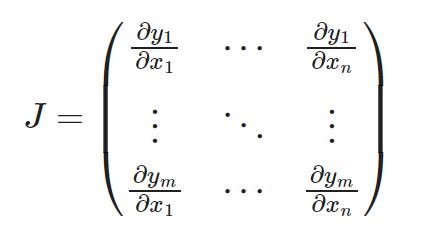
用backward函数和pass v作参数,计算v的转置,v大小=原始tensor大小
c = torch.sqrt(torch.square(a) + torch.square(b))
c.backward(torch.eye(2)) # eye(2) means 2x2 identity matrix
print(a.grad)
输出:
tensor([[-0.8642, 0.0913],
[-0.1666, -0.9710]])
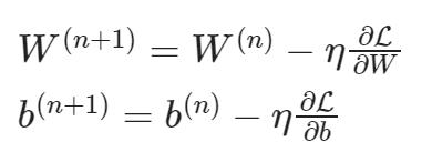
例子0:用梯度下降优化
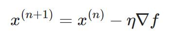
(依塔=学习率lr,▽f=梯度)
x = torch.zeros(2,requires_grad=True)
f = lambda x : (x-torch.tensor([3,-2])).pow(2).sum()
lr = 0.1
15轮梯度下降,逼近最小值点(3,-2):
for i in range(15):
y = f(x)
y.backward()
gr = x.grad
x.data.add_(-lr*gr)
x.grad.zero_()
print("Step {}: x[0]={}, x[1]={}".format(i,x[0],x[1]))
结果:
Step 0: x[0]=0.6000000238418579, x[1]=-0.4000000059604645 Step 1: x[0]=1.0800000429153442, x[1]=-0.7200000286102295 Step 2: x[0]=1.4639999866485596, x[1]=-0.9760000705718994 Step 3: x[0]=1.7711999416351318, x[1]=-1.1808000802993774 Step 4: x[0]=2.0169599056243896, x[1]=-1.3446400165557861 Step 5: x[0]=2.2135679721832275, x[1]=-1.4757120609283447 Step 6: x[0]=2.370854377746582, x[1]=-1.5805696249008179 Step 7: x[0]=2.4966835975646973, x[1]=-1.6644556522369385 Step 8: x[0]=2.597346782684326, x[1]=-1.7315645217895508 Step 9: x[0]=2.677877426147461, x[1]=-1.7852516174316406 Step 10: x[0]=2.7423019409179688, x[1]=-1.8282012939453125 Step 11: x[0]=2.793841600418091, x[1]=-1.8625609874725342 Step 12: x[0]=2.835073232650757, x[1]=-1.8900487422943115 Step 13: x[0]=2.868058681488037, x[1]=-1.912039041519165 Step 14: x[0]=2.894446849822998, x[1]=-1.929631233215332
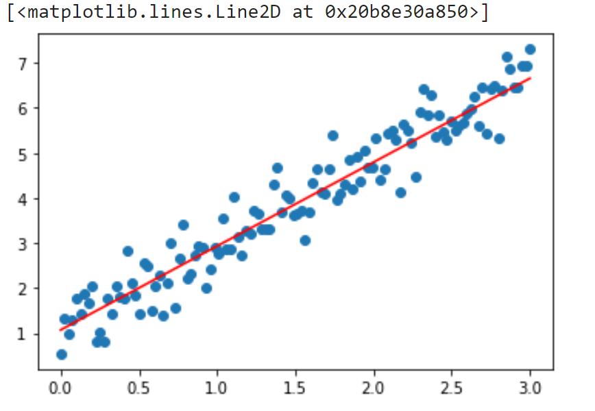
例子1:线性回归
import numpy as np
import matplotlib.pyplot as plt
from sklearn.datasets import make_classification, make_regression
from sklearn.model_selection import train_test_split
import random
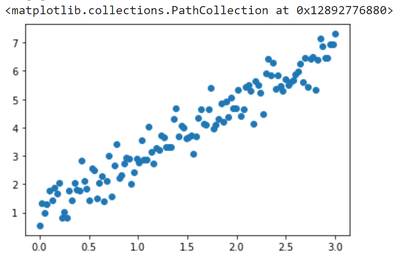
绘图:
np.random.seed(13) # pick the seed for reproducibility - change it to explore the effects of random variations
train_x = np.linspace(0, 3, 120)
train_labels = 2 * train_x + 0.9 + np.random.randn(*train_x.shape) * 0.5
plt.scatter(train_x,train_labels)
定义模型、损失函数:
input_dim = 1output_dim = 1learning_rate = 0.1
# This is our weight matrixw = torch.tensor([100.0],requires_grad=True,dtype=torch.float32)# This is our bias vectorb = torch.zeros(size=(output_dim,),requires_grad=True)
def f(x):
return torch.matmul(x,w) + b
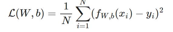
def compute_loss(labels, predictions):
return torch.mean(torch.square(labels - predictions))
输入:
def train_on_batch(x, y):
predictions = f(x)
loss = compute_loss(y, predictions)
loss.backward()
w.data.sub_(learning_rate * w.grad)
b.data.sub_(learning_rate * b.grad)
w.grad.zero_()
b.grad.zero_()
return loss
# Shuffle the data.
indices = np.random.permutation(len(train_x))
features = torch.tensor(train_x[indices],dtype=torch.float32)
labels = torch.tensor(train_labels[indices],dtype=torch.float32)
batch_size = 4
for epoch in range(10):
for i in range(0,len(features),batch_size):
loss = train_on_batch(features[i:i+batch_size].view(-1,1),labels[i:i+batch_size])
print('Epoch %d: last batch loss = %.4f' % (epoch, float(loss)))
输出:Epoch 0: last batch loss = 94.5247
Epoch 1: last batch loss = 9.3428
Epoch 2: last batch loss = 1.4166
Epoch 3: last batch loss = 0.5224
Epoch 4: last batch loss = 0.3807
Epoch 5: last batch loss = 0.3495
Epoch 6: last batch loss = 0.3413
Epoch 7: last batch loss = 0.3390
Epoch 8: last batch loss = 0.3384
Epoch 9: last batch loss = 0.3382
输入:w,b
输出:
(tensor([1.8617], requires_grad=True), tensor([1.0711], requires_grad=True))
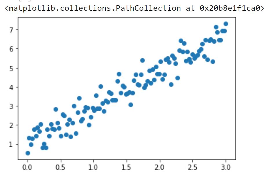
绘图:
plt.scatter(train_x,train_labels)
x = np.array([min(train_x),max(train_x)])
with torch.no_grad():
y = w.numpy()*x+b.numpy()
plt.plot(x,y,color='red')
在GPU里计算(cuda):
device = 'cuda' if torch.cuda.is_available() else 'cpu'
print('Doing computations on '+device)
### Changes here: indicate devicew = torch.tensor([100.0],requires_grad=True,dtype=torch.float32,device=device)b = torch.zeros(size=(output_dim,),requires_grad=True,device=device)
def f(x):
return torch.matmul(x,w) + b
def compute_loss(labels, predictions):
return torch.mean(torch.square(labels - predictions))
def train_on_batch(x, y):
predictions = f(x)
loss = compute_loss(y, predictions)
loss.backward()
w.data.sub_(learning_rate * w.grad)
b.data.sub_(learning_rate * b.grad)
w.grad.zero_()
b.grad.zero_()
return loss
batch_size = 4for epoch in range(10):
for i in range(0,len(features),batch_size):
### Changes here: move data to required device
loss = train_on_batch(features[i:i+batch_size].view(-1,1).to(device),labels[i:i+batch_size].to(device))
print('Epoch %d: last batch loss = %.4f' % (epoch, float(loss)))
输出:
Doing computations on cpu Epoch 0: last batch loss = 94.5247 Epoch 1: last batch loss = 9.3428 Epoch 2: last batch loss = 1.4166 Epoch 3: last batch loss = 0.5224 Epoch 4: last batch loss = 0.3807 Epoch 5: last batch loss = 0.3495 Epoch 6: last batch loss = 0.3413 Epoch 7: last batch loss = 0.3390 Epoch 8: last batch loss = 0.3384 Epoch 9: last batch loss = 0.3382
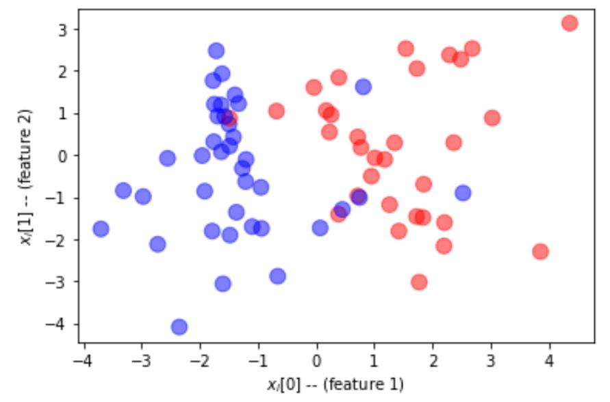
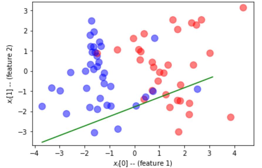
例子2:分类
np.random.seed(0) # pick the seed for reproducibility - change it to explore the effects of random variations
n = 100X, Y = make_classification(n_samples = n, n_features=2,
n_redundant=0, n_informative=2, flip_y=0.1,class_sep=1.5)X = X.astype(np.float32)Y = Y.astype(np.int32)
split = [ 70*n//100, (15+70)*n//100 ]train_x, valid_x, test_x = np.split(X, split)train_labels, valid_labels, test_labels = np.split(Y, split)
def plot_dataset(features, labels, W=None, b=None):
# prepare the plot
fig, ax = plt.subplots(1, 1)
ax.set_xlabel('$x_i[0]$ -- (feature 1)')
ax.set_ylabel('$x_i[1]$ -- (feature 2)')
colors = ['r' if l else 'b' for l in labels]
ax.scatter(features[:, 0], features[:, 1], marker='o', c=colors, s=100, alpha = 0.5)
if W is not None:
min_x = min(features[:,0])
max_x = max(features[:,1])
min_y = min(features[:,1])*(1-.1)
max_y = max(features[:,1])*(1+.1)
cx = np.array([min_x,max_x],dtype=np.float32)
cy = (0.5-W[0]*cx-b)/W[1]
ax.plot(cx,cy,'g')
ax.set_ylim(min_y,max_y)
fig.show()
输入:
plot_dataset(train_x, train_labels)
绘图:
Pytorch训练单层感知器:
一个神经网络有2个in和1个out,W大小=2x1,偏见矢量=1
class Network():
def __init__(self):
self.W = torch.randn(size=(2,1),requires_grad=True)
self.b = torch.zeros(size=(1,),requires_grad=True)
def forward(self,x):
return torch.matmul(x,self.W)+self.b
def zero_grad(self):
self.W.data.zero_()
self.b.data.zero_()
def update(self,lr=0.1):
self.W.data.sub_(lr*self.W.grad)
self.b.data.sub_(lr*self.b)
net = Network()
(用W.data.zero_(),不用W.zero_(),不可以直接调正在Autograd的tensor)
p作网络的输出值,用sigmoid激活函数限制z范围为0-1
pi对应第i个实际类的in,要计算:
以上PyTorch可以直接用binary_cross_entropy_with_logits(),自动算小批量的均值(用binary_crossentropy也行)
def train_on_batch(net, x, y):
z = net.forward(x).flatten()
loss = torch.nn.functional.binary_cross_entropy_with_logits(input=z,target=y)
net.zero_grad()
loss.backward()
net.update()
return loss
# Create a tf.data.Dataset object for easy batched iteration
dataset = torch.utils.data.TensorDataset(torch.tensor(train_x),torch.tensor(train_labels,dtype=torch.float32))
dataloader = torch.utils.data.DataLoader(dataset,batch_size=16)
list(dataloader)[0]
输出:
[tensor([[ 1.5442, 2.5290], [-1.6284, 0.0772], [-1.7141, 2.4770], [-1.4951, 0.7320], [-1.6899, 0.9243], [-0.9474, -0.7681], [ 3.8597, -2.2951], [-1.3944, 1.4300], [ 4.3627, 3.1333], [-1.0973, -1.7011], [-2.5532, -0.0777], [-1.2661, -0.3167], [ 0.3921, 1.8406], [ 2.2091, -1.6045], [ 1.8383, -1.4861], [ 0.7173, -0.9718]]), tensor([1., 0., 0., 0., 0., 0., 1., 0., 1., 0., 0., 0., 1., 1., 1., 1.])]
练15个epochs:
for epoch in range(15):
for (x, y) in dataloader:
loss = train_on_batch(net,x,y)
print('Epoch %d: last batch loss = %.4f' % (epoch, float(loss)))
输出:
Epoch 0: last batch loss = 0.6491
Epoch 1: last batch loss = 0.6064
Epoch 2: last batch loss = 0.5822
Epoch 3: last batch loss = 0.5679
Epoch 4: last batch loss = 0.5592
Epoch 5: last batch loss = 0.5537
Epoch 6: last batch loss = 0.5501
Epoch 7: last batch loss = 0.5478
Epoch 8: last batch loss = 0.5463
Epoch 9: last batch loss = 0.5454
Epoch 10: last batch loss = 0.5447
Epoch 11: last batch loss = 0.5443
Epoch 12: last batch loss = 0.5441
Epoch 13: last batch loss = 0.5439
Epoch 14: last batch loss = 0.5438
调用:
print(net.W,net.b)
输出:
tensor([[ 0.1330], [-0.2810]], requires_grad=True) tensor([0.], requires_grad=True)
绘图:
plot_dataset(train_x,train_labels,net.W.detach().numpy(),net.b.detach().numpy())
计算验证集的准确度:
pred = torch.sigmoid(net.forward(torch.tensor(valid_x)))torch.mean(((pred.view(-1)>0.5)==(torch.tensor(valid_labels)>0.5)).type(torch.float32))
输出:
tensor(0.7333)
torch.nn.Module:定义神经网络
(定义神经网络有两个方法:Module类,Sequential)
module里面可以用标准层次
-
Linear:浓缩线性层次=单层感知器
-
Softmax,Sigmoid,ReLU:对应激活函数
-
其他
用内置Linear层次训练单层感知器:
net = torch.nn.Linear(2,1) # 2 inputs, 1 output
print(list(net.parameters()))
结果:
[Parameter containing: tensor([[-0.0422, 0.1821]], requires_grad=True), Parameter containing: tensor([0.6582], requires_grad=True)]
定义SGD优化器:
optim = torch.optim.SGD(net.parameters(),lr=0.05)
用优化器后的训练循环:
val_x = torch.tensor(valid_x)val_lab = torch.tensor(valid_labels)
for ep in range(10):
for (x,y) in dataloader:
z = net(x).flatten()
loss = torch.nn.functional.binary_cross_entropy_with_logits(z,y)
optim.zero_grad()
loss.backward()
optim.step()
acc = ((torch.sigmoid(net(val_x).flatten())>0.5).float()==val_lab).float().mean()
print(f"Epoch {ep}: last batch loss = {loss}, val acc = {acc}")
输出:
Epoch 0: last batch loss = 0.7596041560173035, val acc = 0.5333333611488342 Epoch 1: last batch loss = 0.6602361798286438, val acc = 0.6000000238418579 Epoch 2: last batch loss = 0.5847358107566833, val acc = 0.6666666865348816 Epoch 3: last batch loss = 0.5263020992279053, val acc = 0.7333333492279053 Epoch 4: last batch loss = 0.48015740513801575, val acc = 0.800000011920929 Epoch 5: last batch loss = 0.4430023431777954, val acc = 0.8666666746139526 Epoch 6: last batch loss = 0.41254672408103943, val acc = 0.8666666746139526 Epoch 7: last batch loss = 0.3871781527996063, val acc = 0.800000011920929 Epoch 8: last batch loss = 0.3657420873641968, val acc = 0.800000011920929 Epoch 9: last batch loss = 0.34739670157432556, val acc = 0.800000011920929
def train(net, dataloader, val_x, val_lab, epochs=10, lr=0.05):
optim = torch.optim.Adam(net.parameters(),lr=lr)
for ep in range(epochs):
for (x,y) in dataloader:
z = net(x).flatten()
loss = torch.nn.functional.binary_cross_entropy_with_logits(z,y)
optim.zero_grad()
loss.backward()
optim.step()
acc = ((torch.sigmoid(net(val_x).flatten())>0.5).float()==val_lab).float().mean()
print(f"Epoch {ep}: last batch loss = {loss}, val acc = {acc}")
net = torch.nn.Linear(2,1)
train(net,dataloader,val_x,val_lab,lr=0.03)
输出:
Epoch 0: last batch loss = 0.48486900329589844, val acc = 0.7333333492279053 Epoch 1: last batch loss = 0.41338109970092773, val acc = 0.800000011920929 Epoch 2: last batch loss = 0.35756850242614746, val acc = 0.800000011920929 Epoch 3: last batch loss = 0.31495171785354614, val acc = 0.800000011920929 Epoch 4: last batch loss = 0.2824164032936096, val acc = 0.800000011920929 Epoch 5: last batch loss = 0.2572754919528961, val acc = 0.800000011920929 Epoch 6: last batch loss = 0.23751722276210785, val acc = 0.800000011920929 Epoch 7: last batch loss = 0.2217157930135727, val acc = 0.800000011920929 Epoch 8: last batch loss = 0.2088666558265686, val acc = 0.800000011920929 Epoch 9: last batch loss = 0.19824868440628052, val acc = 0.800000011920929
把神经网络定义为层次序列:
net = torch.nn.Sequential(torch.nn.Linear(2,5),torch.nn.Sigmoid(),torch.nn.Linear(5,1))
print(net)
输出:
Sequential( (0): Linear(in_features=2, out_features=5, bias=True) (1): Sigmoid() (2): Linear(in_features=5, out_features=1, bias=True) )
输入:
train(net,dataloader,val_x,val_lab)
输出:
Epoch 0: last batch loss = 0.5835739970207214, val acc = 0.800000011920929
Epoch 1: last batch loss = 0.4642275869846344, val acc = 0.800000011920929
Epoch 2: last batch loss = 0.35158076882362366, val acc = 0.800000011920929
Epoch 3: last batch loss = 0.26132312417030334, val acc = 0.800000011920929
Epoch 4: last batch loss = 0.19465585052967072, val acc = 0.800000011920929
Epoch 5: last batch loss = 0.14735405147075653, val acc = 0.800000011920929
Epoch 6: last batch loss = 0.11454981565475464, val acc = 0.800000011920929
Epoch 7: last batch loss = 0.09244414418935776, val acc = 0.800000011920929
Epoch 8: last batch loss = 0.07805468142032623, val acc = 0.800000011920929
Epoch 9: last batch loss = 0.06894762068986893, val acc = 0.800000011920929
将网络定义成类:
class MyNet(torch.nn.Module):
def __init__(self,hidden_size=10,func=torch.nn.Sigmoid()):
super().__init__()
self.fc1 = torch.nn.Linear(2,hidden_size)
self.func = func
self.fc2 = torch.nn.Linear(hidden_size,1)
def forward(self,x):
x = self.fc1(x)
x = self.func(x)
x = self.fc2(x)
return x
net = MyNet(func=torch.nn.ReLU())print(net)
输出:
MyNet( (fc1): Linear(in_features=2, out_features=10, bias=True) (func): ReLU() (fc2): Linear(in_features=10, out_features=1, bias=True) )
输入:
train(net,dataloader,val_x,val_lab,lr=0.005)
输出:
Epoch 0: last batch loss = 0.7821246981620789, val acc = 0.46666666865348816
Epoch 1: last batch loss = 0.7457502484321594, val acc = 0.5333333611488342
Epoch 2: last batch loss = 0.7120334506034851, val acc = 0.5333333611488342
Epoch 3: last batch loss = 0.6811249256134033, val acc = 0.6666666865348816
Epoch 4: last batch loss = 0.6533011794090271, val acc = 0.7333333492279053
Epoch 5: last batch loss = 0.627849280834198, val acc = 0.7333333492279053
Epoch 6: last batch loss = 0.6030643582344055, val acc = 0.800000011920929
Epoch 7: last batch loss = 0.5775002837181091, val acc = 0.800000011920929
Epoch 8: last batch loss = 0.5522137880325317, val acc = 0.8666666746139526
Epoch 9: last batch loss = 0.5250465869903564, val acc = 0.8666666746139526
将网络定义成PyTorch Lightning模块:
import pytorch_lightning as pl
class MyNetPL(pl.LightningModule):
def __init__(self, hidden_size = 10, func = torch.nn.Sigmoid()):
super().__init__()
self.fc1 = torch.nn.Linear(2,hidden_size)
self.func = func
self.fc2 = torch.nn.Linear(hidden_size,1)
self.val_epoch_num = 0 # for logging
def forward(self, x):
x = self.fc1(x)
x = self.func(x)
x = self.fc2(x)
return x
def training_step(self, batch, batch_nb):
x, y = batch
y_res = self(x).view(-1)
loss = torch.nn.functional.binary_cross_entropy_with_logits(y_res, y)
return loss
def configure_optimizers(self):
optimizer = torch.optim.SGD(self.parameters(), lr = 0.005)
return optimizer
def validation_step(self, batch, batch_nb):
x, y = batch
y_res = self(x).view(-1)
val_loss = torch.nn.functional.binary_cross_entropy_with_logits(y_res, y)
print("Epoch ", self.val_epoch_num, ": val loss = ", val_loss.item(), " val acc = ",((torch.sigmoid(y_res.flatten())>0.5).float()==y).float().mean().item(), sep = "")
self.val_epoch_num += 1
valid_dataset = torch.utils.data.TensorDataset(torch.tensor(valid_x),torch.tensor(valid_labels,dtype=torch.float32))valid_dataloader = torch.utils.data.DataLoader(valid_dataset, batch_size = 16)
net = MyNetPL(func=torch.nn.ReLU())trainer = pl.Trainer(max_epochs = 30, log_every_n_steps = 1, accelerator='gpu', devices=1)trainer.fit(model = net, train_dataloaders = dataloader, val_dataloaders = valid_dataloader)
输出:略
扩展阅读:
-
Keras框架实验
-
Keras + TensorFlow2.x框架实验
-
用PyTorch优化器绘制训练数据和验证数据损失函数的图表
-
用 PyTorch优化器解决MNIST分类问题