
Keras + TensorFlow2.x支持动态概念图
简单tensor:
a = tf.constant([[1,2],[3,4]])
print(a)
a = tf.random.normal(shape=(10,3))
print(a)
过程:
tf.Tensor( [[1 2] [3 4]], shape=(2, 2), dtype=int32) tf.Tensor( [[-0.33552304 -1.8252622 -1.8532339 ] [ 1.0871267 -1.2779568 0.5240014 ] [-0.12793781 -1.8618349 -0.9020286 ] [ 0.5948797 0.11144501 -2.0396452 ] [ 0.47620854 1.1726047 -0.4405675 ] [-0.27211484 -0.08985762 -0.03376012] [ 0.64274263 0.53368104 -0.9006528 ] [-0.43745974 -1.0081122 -0.13442488] [ 0.36497566 1.3221073 -1.8739727 ] [ 0.94821155 -0.02817811 1.3563292 ]], shape=(10, 3), dtype=float32)
调用:
print(a-a[0])
print(tf.exp(a)[0].numpy())
输出:
tf.Tensor( [[ 0. 0. 0. ] [ 1.4226497 0.54730535 2.3772354 ] [ 0.20758523 -0.03657269 0.9512053 ] [ 0.93040276 1.9367073 -0.18641126] [ 0.8117316 2.9978669 1.4126664 ] [ 0.0634082 1.7354046 1.8194739 ] [ 0.97826564 2.3589432 0.9525811 ] [-0.1019367 0.81715 1.718809 ] [ 0.7004987 3.1473694 -0.02073872] [ 1.2837346 1.7970841 3.2095633 ]], shape=(10, 3), dtype=float32) [0.71496403 0.16117539 0.15672949]
变量:用assign()和assign_add()
s = tf.Variable(tf.zeros_like(a[0]))
for i in a:
s.assign_add(i)
print(s)
输出:
<tf.Variable 'Variable:0' shape=(3,) dtype=float32, numpy=array([ 2.9411097, -2.9513645, -6.2979555], dtype=float32)>
进一步该写:
tf.reduce_sum(a,axis=0)
输出:
<tf.Tensor: shape=(3,), dtype=float32, numpy=array([ 2.9411097, -2.9513645, -6.2979555], dtype=float32)>
计算梯度:用tf.GradientType()
a = tf.random.normal(shape=(2, 2))b = tf.random.normal(shape=(2, 2))
with tf.GradientTape() as tape:
tape.watch(a) # Start recording the history of operations applied to `a`
c = tf.sqrt(tf.square(a) + tf.square(b)) # Do some math using `a`
# What's the gradient of `c` with respect to `a`?
dc_da = tape.gradient(c, a)
print(dc_da)
输出:
tf.Tensor(
[[ 0.40935674 -0.3495818 ] [ 0.94165146 -0.33209163]], shape=(2, 2), dtype=float32)
线性回归例子:
引入库:
import matplotlib.pyplot as plt
from sklearn.datasets import make_classification, make_regression
from sklearn.model_selection import train_test_split
import random
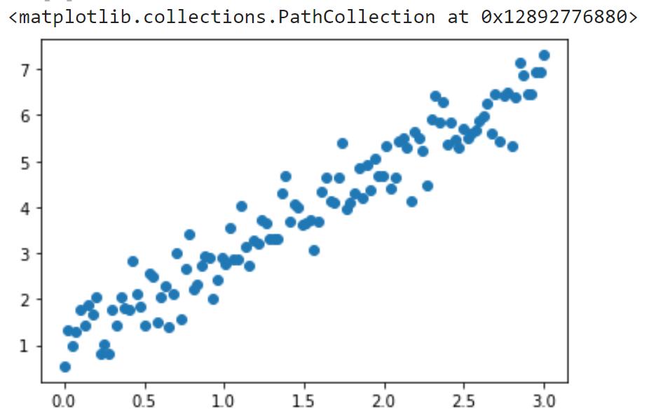
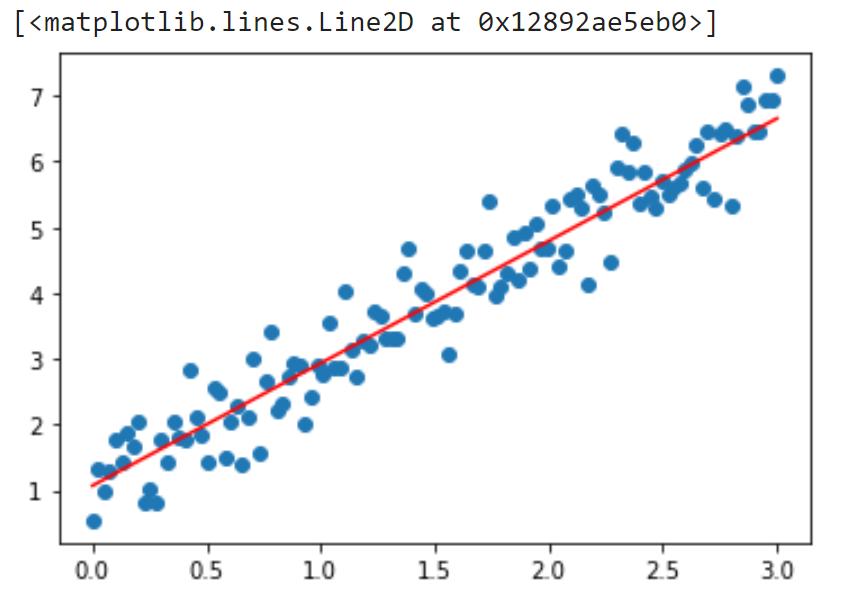
绘图:
np.random.seed(13) # pick the seed for reproducability - change it to explore the effects of random variations
train_x = np.linspace(0, 3, 120)
train_labels = 2 * train_x + 0.9 + np.random.randn(*train_x.shape) * 0.5
plt.scatter(train_x,train_labels)
线性回归线:
损失函数用均方误差表示:
定义模型、损失函数:
input_dim = 1output_dim = 1
learning_rate = 0.1
# This is our weight matrix
w = tf.Variable([[100.0]])# This is our bias vector
b = tf.Variable(tf.zeros(shape=(output_dim,)))
def f(x):
return tf.matmul(x,w) + b
def compute_loss(labels, predictions):
return tf.reduce_mean(tf.square(labels - predictions))
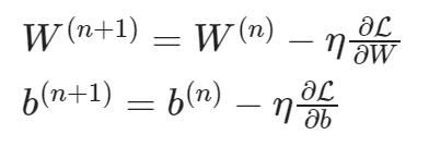
梯度下降:
def train_on_batch(x, y):
with tf.GradientTape() as tape:
predictions = f(x)
loss = compute_loss(y, predictions)
# Note that `tape.gradient` works with a list as well (w, b).
dloss_dw, dloss_db = tape.gradient(loss, [w, b])
w.assign_sub(learning_rate * dloss_dw)
b.assign_sub(learning_rate * dloss_db)
return loss
训练:做epochs,拆解成小批量
# Shuffle the data.
indices = np.random.permutation(len(train_x))
features = tf.constant(train_x[indices],dtype=tf.float32)
labels = tf.constant(train_labels[indices],dtype=tf.float32)
batch_size = 4
for epoch in range(10):
for i in range(0,len(features),batch_size):
loss = train_on_batch(tf.reshape(features[i:i+batch_size],(-1,1)),tf.reshape(labels[i:i+batch_size],(-1,1)))
print('Epoch %d: last batch loss = %.4f' % (epoch, float(loss)))
过程:
Epoch 0: last batch loss = 94.5247 Epoch 1: last batch loss = 9.3428 Epoch 2: last batch loss = 1.4166 Epoch 3: last batch loss = 0.5224 Epoch 4: last batch loss = 0.3807 Epoch 5: last batch loss = 0.3495 Epoch 6: last batch loss = 0.3413 Epoch 7: last batch loss = 0.3390 Epoch 8: last batch loss = 0.3384 Epoch 9: last batch loss = 0.3382
成功训练接近真实参数的模型,但由于噪声和优化限制,结果与原始值有误差,参数应该无线接近W=2,b
=1才对。
绘图:
plt.scatter(train_x,train_labels)
x = np.array([min(train_x),max(train_x)])
y = w.numpy()[0,0]*x+b.numpy()[0]
plt.plot(x,y,color='red')
在GPU上运行代码时,在CPU和GPU间反复pass迭代
@tf.functiondef train_on_batch(x, y):
with tf.GradientTape() as tape:
predictions = f(x)
loss = compute_loss(y, predictions)
# Note that `tape.gradient` works with a list as well (w, b).
dloss_dw, dloss_db = tape.gradient(loss, [w, b])
w.assign_sub(learning_rate * dloss_dw)
b.assign_sub(learning_rate * dloss_db)
return loss
数据集API:
w.assign([[10.0]])b.assign([0.0])
# Create a tf.data.Dataset object for easy batched iterationdataset = tf.data.Dataset.from_tensor_slices((train_x.astype(np.float32), train_labels.astype(np.float32)))dataset = dataset.shuffle(buffer_size=1024).batch(256)
for epoch in range(10):
for step, (x, y) in enumerate(dataset):
loss = train_on_batch(tf.reshape(x,(-1,1)), tf.reshape(y,(-1,1)))
print('Epoch %d: last batch loss = %.4f' % (epoch, float(loss)))
过程:
Epoch 0: last batch loss = 173.4585
Epoch 1: last batch loss = 13.8459
Epoch 2: last batch loss = 4.5407
Epoch 3: last batch loss = 3.7364
Epoch 4: last batch loss = 3.4334
Epoch 5: last batch loss = 3.1790
Epoch 6: last batch loss = 2.9458
Epoch 7: last batch loss = 2.7311
Epoch 8: last batch loss = 2.5332
Epoch 9: last batch loss = 2.3508
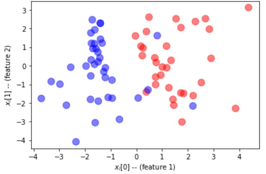
分类器:
np.random.seed(0) # pick the seed for reproducibility - change it to explore the effects of random variations
n = 100
X, Y = make_classification(n_samples = n, n_features=2, n_redundant=0, n_informative=2, flip_y=0.05,class_sep=1.5)
X = X.astype(np.float32)
Y = Y.astype(np.int32)
split = [ 70*n//100, (15+70)*n//100 ]
train_x, valid_x, test_x = np.split(X, split)
train_labels, valid_labels, test_labels = np.split(Y, split)
def plot_dataset(features, labels, W=None, b=None):
# prepare the plot
fig, ax = plt.subplots(1, 1)
ax.set_xlabel('$x_i[0]$ -- (feature 1)')
ax.set_ylabel('$x_i[1]$ -- (feature 2)')
colors = ['r' if l else 'b' for l in labels]
ax.scatter(features[:, 0], features[:, 1], marker='o', c=colors, s=100, alpha = 0.5)
if W is not None:
min_x = min(features[:,0])
max_x = max(features[:,1])
min_y = min(features[:,1])*(1-.1)
max_y = max(features[:,1])*(1+.1)
cx = np.array([min_x,max_x],dtype=np.float32)
cy = (0.5-W[0]*cx-b)/W[1]
ax.plot(cx,cy,'g')
ax.set_ylim(min_y,max_y)
fig.show()
绘图:
plot_dataset(train_x, train_labels)
标准化:
train_x_norm = (train_x-np.min(train_x)) / (np.max(train_x)-np.min(train_x))
valid_x_norm = (valid_x-np.min(train_x)) / (np.max(train_x)-np.min(train_x))
test_x_norm = (test_x-np.min(train_x)) / (np.max(train_x)-np.min(train_x))
训练单层感知器:
W = tf.Variable(tf.random.normal(shape=(2,1)),dtype=tf.float32)
b = tf.Variable(tf.zeros(shape=(1,),dtype=tf.float32))
learning_rate = 0.1
@tf.function
def train_on_batch(x, y):
with tf.GradientTape() as tape:
z = tf.matmul(x, W) + b
loss = tf.reduce_mean(tf.nn.sigmoid_cross_entropy_with_logits(labels=y,logits=z))
dloss_dw, dloss_db = tape.gradient(loss, [W, b])
W.assign_sub(learning_rate * dloss_dw)
b.assign_sub(learning_rate * dloss_db)
return loss
用16元素的小批量,少量训练epochs:
# Create a tf.data.Dataset object for easy batched iterationdataset = tf.data.Dataset.from_tensor_slices((train_x_norm.astype(np.float32), train_labels.astype(np.float32)))dataset = dataset.shuffle(128).batch(2)
for epoch in range(10):
for step, (x, y) in enumerate(dataset):
loss = train_on_batch(x, tf.expand_dims(y,1))
print('Epoch %d: last batch loss = %.4f' % (epoch, float(loss)))
过程:
Epoch 0: last batch loss = 0.3823 Epoch 1: last batch loss = 0.5243 Epoch 2: last batch loss = 0.4510 Epoch 3: last batch loss = 0.3261 Epoch 4: last batch loss = 0.4177 Epoch 5: last batch loss = 0.3323 Epoch 6: last batch loss = 0.6294 Epoch 7: last batch loss = 0.6334 Epoch 8: last batch loss = 0.2571 Epoch 9: last batch loss = 0.3425
pred = tf.matmul(test_x,W)+b
fig,ax = plt.subplots(1,2)ax[0].scatter(test_x[:,0],test_x[:,1],c=pred[:,0]>0.5)
ax[1].scatter(test_x[:,0],test_x[:,1],c=valid_labels)
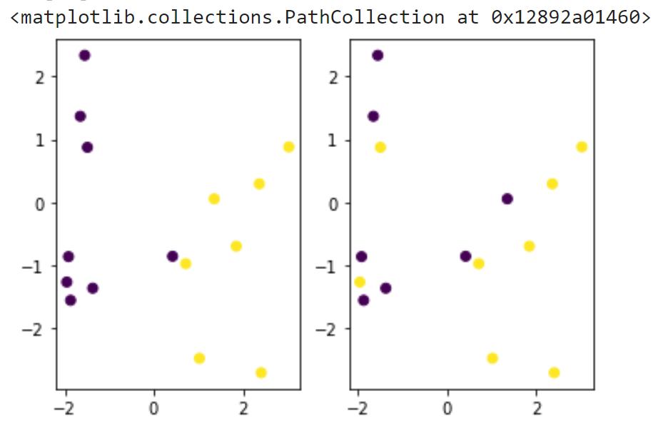
计算准确度:将boolean强转float,计算平均值
tf.reduce_mean(tf.cast(((pred[0]>0.5)==test_labels),tf.float32))
输出:
<tf.Tensor: shape=(), dtype=float32, numpy=0.46666667>
用TensorFlow/Keras的优化器:
optimizer = tf.keras.optimizers.Adam(0.01)
W = tf.Variable(tf.random.normal(shape=(2,1)))b = tf.Variable(tf.zeros(shape=(1,),dtype=tf.float32))
@tf.functiondef train_on_batch(x, y):
vars = [W, b]
with tf.GradientTape() as tape:
z = tf.sigmoid(tf.matmul(x, W) + b)
loss = tf.reduce_mean(tf.keras.losses.binary_crossentropy(z,y))
correct_prediction = tf.equal(tf.round(y), tf.round(z))
acc = tf.reduce_mean(tf.cast(correct_prediction, tf.float32))
grads = tape.gradient(loss, vars)
optimizer.apply_gradients(zip(grads,vars))
return loss,acc
for epoch in range(20):
for step, (x, y) in enumerate(dataset):
loss,acc = train_on_batch(tf.reshape(x,(-1,2)), tf.reshape(y,(-1,1)))
print('Epoch %d: last batch loss = %.4f, acc = %.4f' % (epoch, float(loss),acc))
过程:
Epoch 0: last batch loss = 4.7787, acc = 1.0000 Epoch 1: last batch loss = 8.4343, acc = 0.5000 Epoch 2: last batch loss = 8.3255, acc = 0.5000 Epoch 3: last batch loss = 7.5579, acc = 0.5000 Epoch 4: last batch loss = 6.5254, acc = 0.5000 Epoch 5: last batch loss = 7.3800, acc = 0.5000 Epoch 6: last batch loss = 7.7586, acc = 0.5000 Epoch 7: last batch loss = 10.4724, acc = 0.0000 Epoch 8: last batch loss = 9.4423, acc = 0.5000 Epoch 9: last batch loss = 4.1888, acc = 1.0000 Epoch 10: last batch loss = 11.2127, acc = 0.0000 Epoch 11: last batch loss = 9.0417, acc = 0.5000 Epoch 12: last batch loss = 7.9847, acc = 0.5000 Epoch 13: last batch loss = 3.7879, acc = 1.0000 Epoch 14: last batch loss = 6.8455, acc = 0.5000 Epoch 15: last batch loss = 6.5204, acc = 0.5000 Epoch 16: last batch loss = 9.2386, acc = 0.5000 Epoch 17: last batch loss = 6.2447, acc = 0.5000 Epoch 18: last batch loss = 3.9107, acc = 1.0000 Epoch 19: last batch loss = 5.7645, acc = 1.0000
Keras的功能API:定义keras.Input,pass迭代后计算输出,以此定义input变换成output的模型
inputs = tf.keras.Input(shape=(2,))z = tf.keras.layers.Dense(1,kernel_initializer='glorot_uniform',activation='sigmoid')(inputs)model = tf.keras.models.Model(inputs,z)
model.compile(tf.keras.optimizers.Adam(0.1),'binary_crossentropy',['accuracy'])model.summary()h = model.fit(train_x_norm,train_labels,batch_size=8,epochs=15)
过程:略
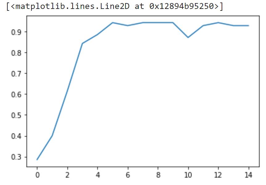
绘图:
plt.plot(h.history['accuracy'])
Sequential API:
model = tf.keras.models.Sequential()
model.add(tf.keras.layers.Dense(5,activation='sigmoid',input_shape=(2,)))
model.add(tf.keras.layers.Dense(1,activation='sigmoid'))
model.compile(tf.keras.optimizers.Adam(0.1),'binary_crossentropy',['accuracy'])
model.summary()
model.fit(train_x_norm,train_labels,validation_data=(test_x_norm,test_labels),batch_size=8,epochs=15)
过程:略
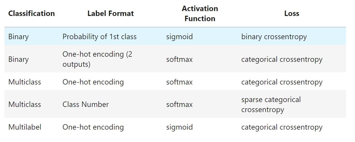
分类损失函数:
-
1个output的,如二分分类,用sigmoid激活函数(多类分类-softmax)
-
output类作one-hot编译,为交叉熵损失;还有数字就是稀疏交叉熵损失;二分分类用二分交叉熵(对数损失)
-
多标签分类:同个物体属于不同类,用one-hot编码,然后sigmoid激活函数
扩展阅读:
-
用TF/Keras优化器绘制训练数据和验证数据损失函数的图表
-
用TF/Keras优化器解决MNIST分类问题
-
用Keras训练MNIST分类器