
引入库:
%matplotlib nbagg
import matplotlib.pyplot as plt
from matplotlib import gridspec
from sklearn.datasets import make_classification
import numpy as np
# pick the seed for reproducibility - change it to explore the effects of random variations
np.random.seed(0)import random
创建两个参数的数据集:
n = 100
X, Y = make_classification(n_samples = n, n_features=2, n_redundant=0, n_informative=2, flip_y=0.2)
X = X.astype(np.float32)
Y = Y.astype(np.int32)
# Split into train and test dataset
train_x, test_x = np.split(X, [n*8//10])
train_labels, test_labels = np.split(Y, [n*8//10])
def plot_dataset(suptitle, features, labels):
# prepare the plot
fig, ax = plt.subplots(1, 1)
#pylab.subplots_adjust(bottom=0.2, wspace=0.4)
fig.suptitle(suptitle, fontsize = 16)
ax.set_xlabel('$x_i[0]$ -- (feature 1)')
ax.set_ylabel('$x_i[1]$ -- (feature 2)')
colors = ['r' if l else 'b' for l in labels]
ax.scatter(features[:, 0], features[:, 1], marker='o', c=colors, s=100, alpha = 0.5)
fig.show()
绘图:
plot_dataset('Scatterplot of the training data', train_x, train_labels)plt.show()
print(train_x[:5])
print(train_labels[:5])
输出:
[[ 1.3382818 -0.98613256]
[ 0.5128146 0.43299454]
[-0.4473693 -0.2680512 ]
[-0.9865851 -0.28692 ]
[-1.0693829 0.41718036]]
[1 1 0 0 0]
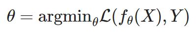
机器学习模型评估标准:
用loss function 损失函数(L)评估的时候,模型解决的问题数也多,效果越好,损失函数就越低
回归损失函数:
-
用绝对误差:
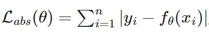
-
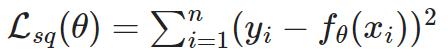
用平均平方差:
# helper function for plotting various loss functionsdef plot_loss_functions(suptitle, functions, ylabels, xlabel):
fig, ax = plt.subplots(1,len(functions), figsize=(9, 3))
plt.subplots_adjust(bottom=0.2, wspace=0.4)
fig.suptitle(suptitle)
for i, fun in enumerate(functions):
ax[i].set_xlabel(xlabel)
if len(ylabels) > i:
ax[i].set_ylabel(ylabels[i])
ax[i].plot(x, fun)
plt.show()
绘图:
x = np.linspace(-2, 2, 101)plot_loss_functions(
suptitle = 'Common loss functions for regression',
functions = [np.abs(x), np.power(x, 2)],
ylabels = ['$\mathcal{L}_{abs}}$ (absolute loss)',
'$\mathcal{L}_{sq}$ (squared loss)'],
xlabel = '$y - f(x_i)$')
分类的损失函数:
0-1损失: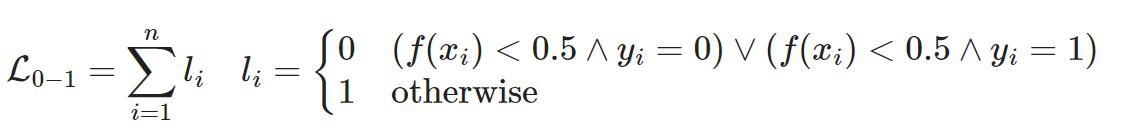 ,计算正确分类数量,但是不展示距离
对数损失: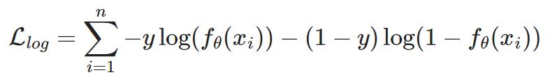
x = np.linspace(0,1,100)def zero_one(d):
if d < 0.5:
return 0
return 1zero_one_v = np.vectorize(zero_one)
def logistic_loss(fx):
# assumes y == 1
return -np.log(fx)
绘图:
plot_loss_functions(suptitle = 'Common loss functions for classification (class=1)',
functions = [zero_one_v(x), logistic_loss(x)],
ylabels = ['$\mathcal{L}_{0-1}}$ (0-1 loss)',
'$\mathcal{L}_{log}$ (logistic loss)'],
xlabel = '$p$')
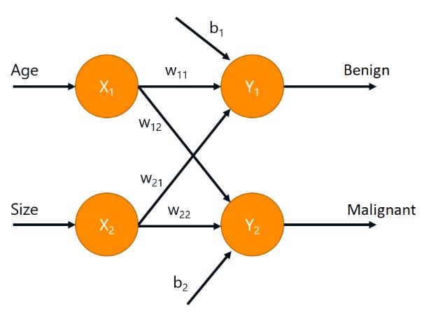
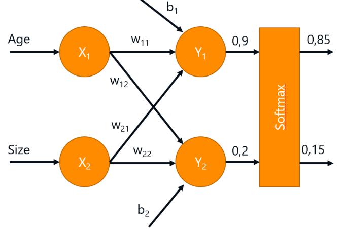
神经网络架构(肿瘤为例):2个output=2个class,2个class取max=正确答案
 ,
,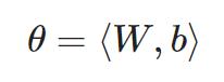
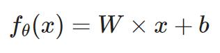
x=input,W和b存在layer class中,初始化W=随机值(打破对称性,防止学习相同),初始化b=0(保证训练初期网络稳定性)
class Linear:
def __init__(self,nin,nout):
self.W = np.random.normal(0, 1.0/np.sqrt(nin), (nout, nin))
self.b = np.zeros((1,nout))
def forward(self, x):
return np.dot(x, self.W.T) + self.b
net = Linear(2,2)net.forward(train_x[0:5])
输出:
array([[ 1.77202116, -0.25384488],
[ 0.28370828, -0.39610552],
[-0.30097433, 0.30513182],
[-0.8120485 , 0.56079421],
[-1.23519653, 0.3394973 ]])
softmax函数:输出转成概率
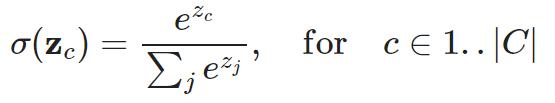
class Softmax:
def forward(self,z):
zmax = z.max(axis=1,keepdims=True)
expz = np.exp(z-zmax)
Z = expz.sum(axis=1,keepdims=True)
return expz / Z
softmax = Softmax()
softmax.forward(net.forward(train_x[0:10]))
输出:
array([[0.88348621, 0.11651379], [0.66369714, 0.33630286], [0.35294795, 0.64705205], [0.20216095, 0.79783905], [0.17154828, 0.82845172], [0.24279153, 0.75720847], [0.18915732, 0.81084268], [0.17282951, 0.82717049], [0.13897531, 0.86102469], [0.72746882, 0.27253118]])
交叉熵损失函数:
损失函数是对数函数,也算是交叉熵损失,交叉熵损失可以算两个概率分布的距离
有两个分布,一个是概率输出,一个是one-hot分布(找p1对应的类c);网络对预期类返回p1,则交叉熵损失=0;p越接近0,交叉熵损失也高
def plot_cross_ent():
p = np.linspace(0.01, 0.99, 101) # estimated probability p(y|x)
cross_ent_v = np.vectorize(cross_ent)
f3, ax = plt.subplots(1,1, figsize=(8, 3))
l1, = plt.plot(p, cross_ent_v(p, 1), 'r--')
l2, = plt.plot(p, cross_ent_v(p, 0), 'r-')
plt.legend([l1, l2], ['$y = 1$', '$y = 0$'], loc = 'upper center', ncol = 2)
plt.xlabel('$\hat{p}(y|x)$', size=18)
plt.ylabel('$\mathcal{L}_{CE}$', size=18)
plt.show()
def cross_ent(prediction, ground_truth):
t = 1 if ground_truth > 0.5 else 0
return -t * np.log(prediction) - (1 - t) * np.log(1 - prediction)
plot_cross_ent()
交叉熵损失可再分层,然后forward()就得有两个输入参数,前置层的输出=p,预期类=y
class CrossEntropyLoss:
def forward(self,p,y):
self.p = p
self.y = y
p_of_y = p[np.arange(len(y)), y]
log_prob = np.log(p_of_y)
return -log_prob.mean() # average over all input samples(要算平均值,交叉熵损失是按单个输入矢量算的,多个矢量要算平均)
cross_ent_loss = CrossEntropyLoss()
p = softmax.forward(net.forward(train_x[0:10]))
cross_ent_loss.forward(p,train_labels[0:10])
输出:
1.429664938969559
计算训练集的损失:
z = net.forward(train_x[0:10])
p = softmax.forward(z)
loss = cross_ent_loss.forward(p,train_labels[0:10])
print(loss)
输出:1.429664938969559
训练集的损失函数: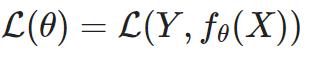
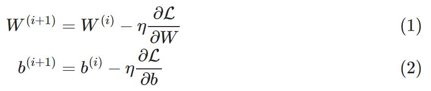
损失最小化: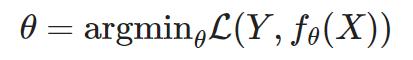
(梯度下降=计算损失函数的梯度)
minibatches小批量:实战应用只要算小批量的梯度·,不用算整个训练集
SGD随机梯度下降算法:每个小批量=子集,子集每次都是随机的
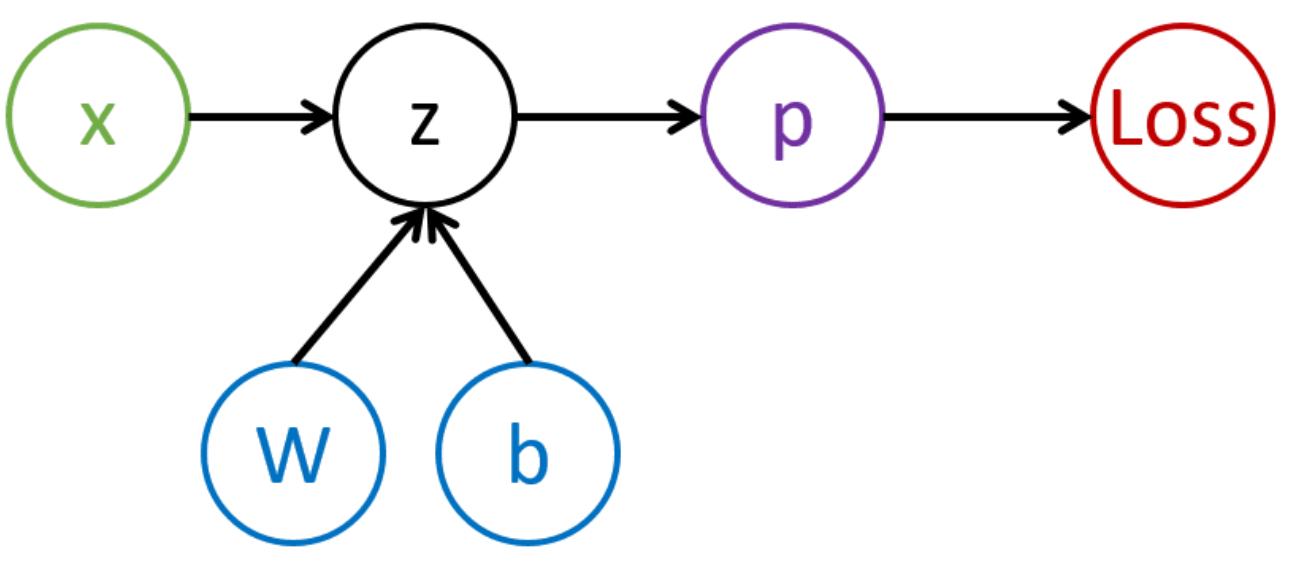
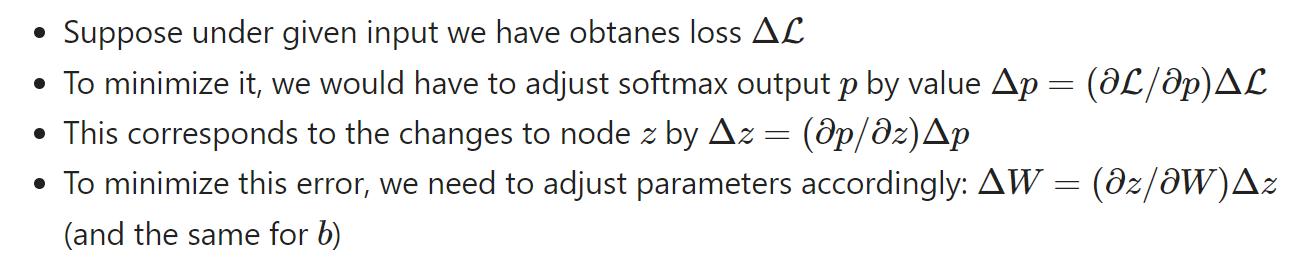
反向传播:输出误差反向传播到误差函数的参数中
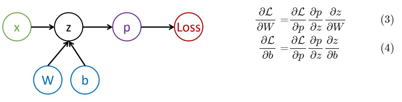
计算过程:
神经训练两个迭代:
-
前向迭代:计算输入小批量的损失
-
后向迭代:按照概念图反向传播将误差最小化
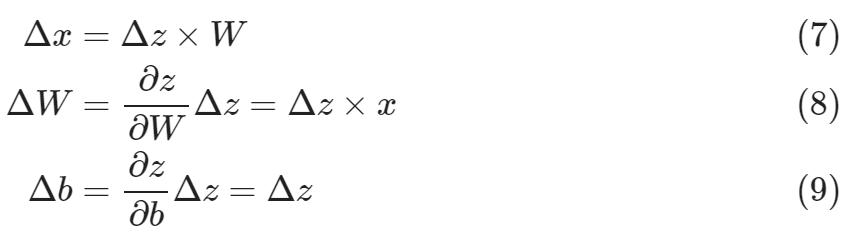
后向传播步骤:算整个小批量的,要更新△W和△b
所有层次求导(z=xW+b;误差=z)
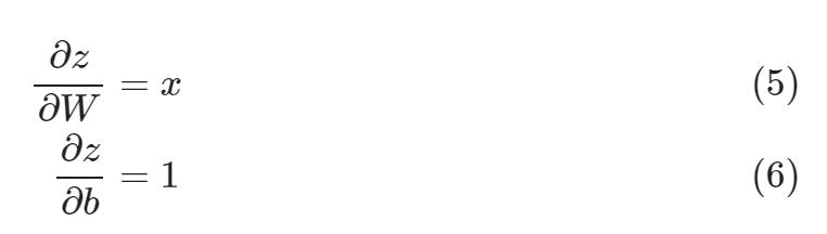
补偿某层次输出的△z要更新W:
class Linear:
def __init__(self,nin,nout):
self.W = np.random.normal(0, 1.0/np.sqrt(nin), (nout, nin))
self.b = np.zeros((1,nout))
self.dW = np.zeros_like(self.W)
self.db = np.zeros_like(self.b)
def forward(self, x):
self.x=x
return np.dot(x, self.W.T) + self.b
def backward(self, dz):
dx = np.dot(dz, self.W)
dW = np.dot(dz.T, self.x)
db = dz.sum(axis=0)
self.dW = dW
self.db = db
return dx
def update(self,lr):
self.W -= lr*self.dW
self.b -= lr*self.db
其他层次的backward函数:
class Softmax:
def forward(self,z):
self.z = z
zmax = z.max(axis=1,keepdims=True)
expz = np.exp(z-zmax)
Z = expz.sum(axis=1,keepdims=True)
return expz / Z
def backward(self,dp):
p = self.forward(self.z)
pdp = p * dp
return pdp - p * pdp.sum(axis=1, keepdims=True)
class CrossEntropyLoss:
def forward(self,p,y):
self.p = p
self.y = y
p_of_y = p[np.arange(len(y)), y]
log_prob = np.log(p_of_y)
return -log_prob.mean()
def backward(self,loss):
dlog_softmax = np.zeros_like(self.p)
dlog_softmax[np.arange(len(self.y)), self.y] -= 1.0/len(self.y)
return dlog_softmax / self.p
训练模型(epoch轮次=训练集的一次完整迭代,不是iteration):
lin = Linear(2,2)
softmax = Softmax()
cross_ent_loss = CrossEntropyLoss()
learning_rate = 0.1
pred = np.argmax(lin.forward(train_x),axis=1)
acc = (pred==train_labels).mean()
print("Initial accuracy: ",acc)
batch_size=4
for i in range(0,len(train_x),batch_size):
xb = train_x[i:i+batch_size]
yb = train_labels[i:i+batch_size]
# forward pass
z = lin.forward(xb)
p = softmax.forward(z)
loss = cross_ent_loss.forward(p,yb)
# backward pass
dp = cross_ent_loss.backward(loss)
dz = softmax.backward(dp)
dx = lin.backward(dz)
lin.update(learning_rate)
pred = np.argmax(lin.forward(train_x),axis=1)
acc = (pred==train_labels).mean()
print("Final accuracy: ",acc)
输出:准确率提升到80%
Initial accuracy: 0.725
Final accuracy: 0.825
神经类:
class Net:
def __init__(self):
self.layers = []
def add(self,l):
self.layers.append(l)
def forward(self,x):
for l in self.layers:
x = l.forward(x)
return x
def backward(self,z):
for l in self.layers[::-1]:
z = l.backward(z)
return z
def update(self,lr):
for l in self.layers:
if 'update' in l.__dir__():
l.update(lr)
net = Net()net.add(Linear(2,2))net.add(Softmax())loss = CrossEntropyLoss()
def get_loss_acc(x,y,loss=CrossEntropyLoss()):
p = net.forward(x)
l = loss.forward(p,y)
pred = np.argmax(p,axis=1)
acc = (pred==y).mean()
return l,acc
print("Initial loss={}, accuracy={}: ".format(*get_loss_acc(train_x,train_labels)))
def train_epoch(net, train_x, train_labels, loss=CrossEntropyLoss(), batch_size=4, lr=0.1):
for i in range(0,len(train_x),batch_size):
xb = train_x[i:i+batch_size]
yb = train_labels[i:i+batch_size]
p = net.forward(xb)
l = loss.forward(p,yb)
dp = loss.backward(l)
dx = net.backward(dp)
net.update(lr)
train_epoch(net,train_x,train_labels)
print("Final loss={}, accuracy={}: ".format(*get_loss_acc(train_x,train_labels)))
print("Test loss={}, accuracy={}: ".format(*get_loss_acc(test_x,test_labels)))
输出:
Initial loss=0.6212072429381601, accuracy=0.6875:
Final loss=0.44369925927417986, accuracy=0.8:
Test loss=0.4767711377257787, accuracy=0.85:
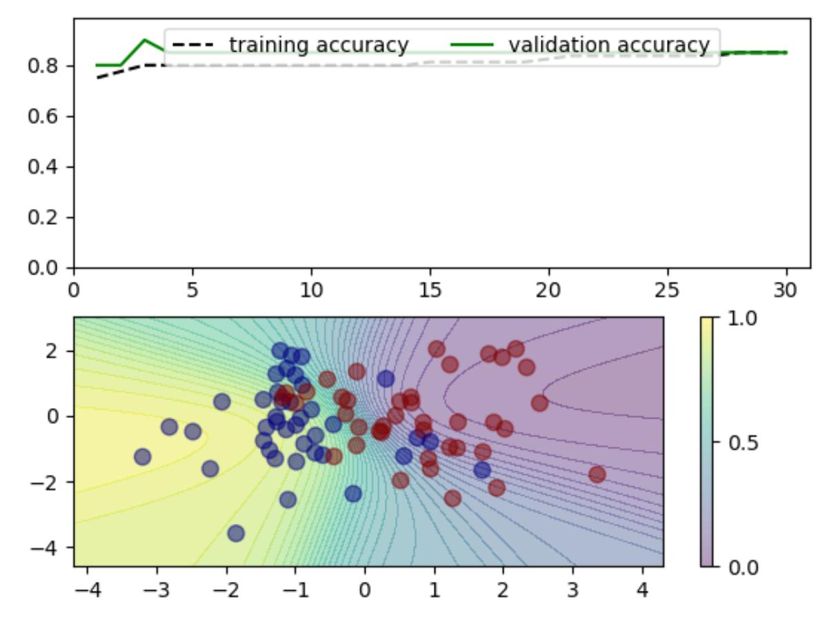
绘训练过程的图:
def train_and_plot(n_epoch, net, loss=CrossEntropyLoss(), batch_size=4, lr=0.1):
fig, ax = plt.subplots(2, 1)
ax[0].set_xlim(0, n_epoch + 1)
ax[0].set_ylim(0,1)
train_acc = np.empty((n_epoch, 3))
train_acc[:] = np.NAN
valid_acc = np.empty((n_epoch, 3))
valid_acc[:] = np.NAN
for epoch in range(1, n_epoch + 1):
train_epoch(net,train_x,train_labels,loss,batch_size,lr)
tloss, taccuracy = get_loss_acc(train_x,train_labels,loss)
train_acc[epoch-1, :] = [epoch, tloss, taccuracy]
vloss, vaccuracy = get_loss_acc(test_x,test_labels,loss)
valid_acc[epoch-1, :] = [epoch, vloss, vaccuracy]
ax[0].set_ylim(0, max(max(train_acc[:, 2]), max(valid_acc[:, 2])) * 1.1)
plot_training_progress(train_acc[:, 0], (train_acc[:, 2],
valid_acc[:, 2]), fig, ax[0])
plot_decision_boundary(net, fig, ax[1])
fig.canvas.draw()
fig.canvas.flush_events()
return train_acc, valid_acc
import matplotlib.cm as cm
def plot_decision_boundary(net, fig, ax):
draw_colorbar = True
# remove previous plot
while ax.collections:
ax.collections.pop()
draw_colorbar = False
# generate countour grid
x_min, x_max = train_x[:, 0].min() - 1, train_x[:, 0].max() + 1
y_min, y_max = train_x[:, 1].min() - 1, train_x[:, 1].max() + 1
xx, yy = np.meshgrid(np.arange(x_min, x_max, 0.1),
np.arange(y_min, y_max, 0.1))
grid_points = np.c_[xx.ravel().astype('float32'), yy.ravel().astype('float32')]
n_classes = max(train_labels)+1
while train_x.shape[1] > grid_points.shape[1]:
# pad dimensions (plot only the first two)
grid_points = np.c_[grid_points,
np.empty(len(xx.ravel())).astype('float32')]
grid_points[:, -1].fill(train_x[:, grid_points.shape[1]-1].mean())
# evaluate predictions
prediction = np.array(net.forward(grid_points))
# for two classes: prediction difference
if (n_classes == 2):
Z = np.array([0.5+(p[0]-p[1])/2.0 for p in prediction]).reshape(xx.shape)
else:
Z = np.array([p.argsort()[-1]/float(n_classes-1) for p in prediction]).reshape(xx.shape)
# draw contour
levels = np.linspace(0, 1, 40)
cs = ax.contourf(xx, yy, Z, alpha=0.4, levels = levels)
if draw_colorbar:
fig.colorbar(cs, ax=ax, ticks = [0, 0.5, 1])
c_map = [cm.jet(x) for x in np.linspace(0.0, 1.0, n_classes) ]
colors = [c_map[l] for l in train_labels]
ax.scatter(train_x[:, 0], train_x[:, 1], marker='o', c=colors, s=60, alpha = 0.5
def plot_training_progress(x, y_data, fig, ax):
styles = ['k--', 'g-']
# remove previous plot
while ax.lines:
ax.lines.pop()
# draw updated lines
for i in range(len(y_data)):
ax.plot(x, y_data[i], styles[i])
ax.legend(ax.lines, ['training accuracy', 'validation accuracy'],
loc='upper center', ncol = 2)
%matplotlib nbagg
net = Net()net.add(Linear(2,2))net.add(Softmax())
res = train_and_plot(30,net,lr=0.005)
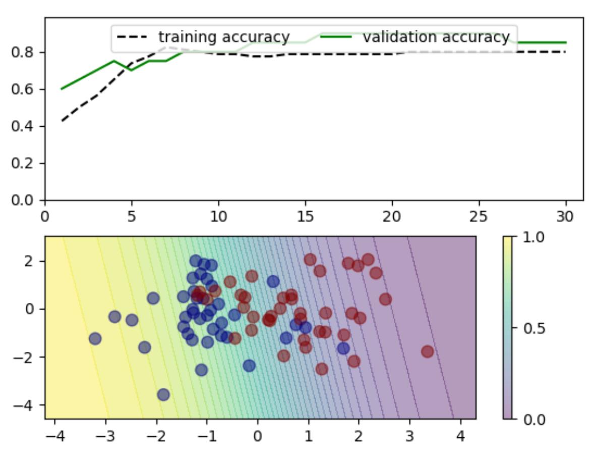
多层次模型:要非线性激活函数tanh(避免多个线性层叠加等于单层=线性变换组合是线性变换,不管叠多少层都是一个线性变换,无法描述非线性关系)
class Tanh:
def forward(self,x):
y = np.tanh(x)
self.y = y
return y
def backward(self,dy):
return (1.0-self.y**2)*dy
多层模型作为reacher
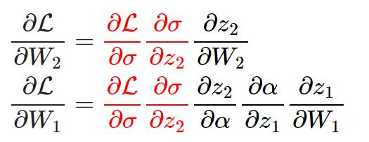
多层感知器表示复杂函数的数学逻辑:

(α=非线性激活函数,σ=softmax函数)
net = Net()
net.add(Linear(2,10))
net.add(Tanh())
net.add(Linear(10,2))
net.add(Softmax())
loss = CrossEntropyLoss()
res = train_and_plot(30,net,lr=0.01)
结论:不要经常用多层模型,因为过度拟合了