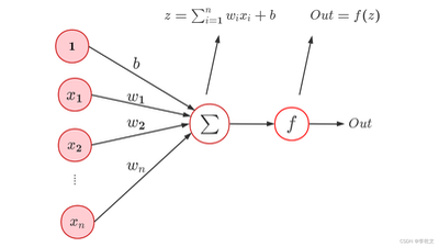
感知器是最简单的神经网络,如图为感知器的基本结构:

感知器可解决二元分类问题,正负分类。
引入库:
import pylab

from matplotlib import gridspec

from sklearn.datasets import make_classification

import numpy as np

from ipywidgets

import interact, interactive, fixed

import ipywidgets as widgets

import pickle

import os

import gzip


# pick the seed for reproducability - change it to explore the effects of random variations

np.random.seed(1)import random
分析肿瘤:良性1,恶性-1
n = 50X, Y = make_classification(n_samples = n, n_features=2, n_redundant=0, n_informative=2, flip_y=0)

Y = Y*2-1 # convert initial 0/1 values into -1/1

X = X.astype(np.float32);

Y = Y.astype(np.int32) # features - float, label - int
调用:
# Split the dataset into training and test

train_x, test_x = np.split(X, [ n*8//10])

train_labels, test_labels = np.split(Y, [n*8//10])

print("Features:\n",train_x[0:4])

print("Labels:\n",train_labels[0:4])
输出:
Features:

[[-1.7441838 -1.3952037 ]

[ 2.5921783 -0.08124504]

[ 0.9218062 0.91789985]

[-0.8437018 -0.18738253]]

Labels:

[-1 -1 1 -1]
绘图:
def plot_dataset(suptitle, features, labels):
# prepare the plot
fig, ax = pylab.subplots(1, 1)
#pylab.subplots_adjust(bottom=0.2, wspace=0.4)
fig.suptitle(suptitle, fontsize = 16)
ax.set_xlabel('$x_i[0]$ -- (feature 1)')
ax.set_ylabel('$x_i[1]$ -- (feature 2)')
colors = ['r' if l>0 else 'b' for l in labels]
ax.scatter(features[:, 0], features[:, 1], marker='o', c=colors, s=100, alpha = 0.5)
fig.show()
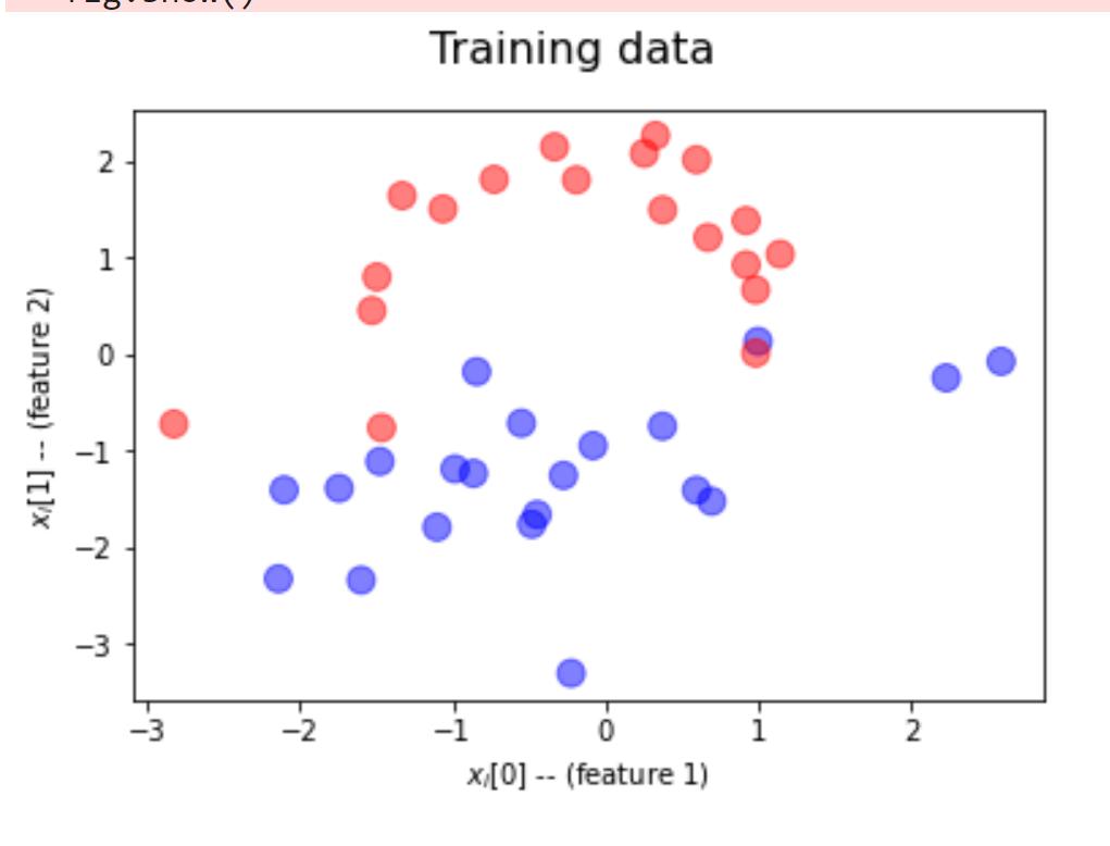
plot_dataset('Training data', train_x, train_labels)
结果:
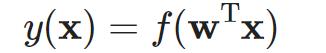
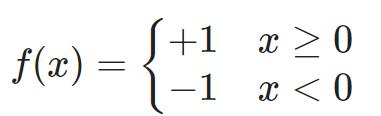
感知器公式:
输入:
pos_examples = np.array([ [t[0], t[1], 1]

for i,t in enumerate(train_x)
   if train_labels[i]>0])
      neg_examples = np.array([ [t[0], t[1], 1]
        for i,t in enumerate(train_x)
           if train_labels[i]<0])print(pos_examples[0:3])
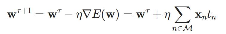
训练算法:
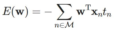
t是-1和+1,M=mistake=错误分类的例子
梯度下降,设w0是随机数,每一步训练都要用E的梯度调整w,依塔=学习率,τ迭代数
def train(positive_examples, negative_examples, num_iterations = 100):

   num_dims = positive_examples.shape[1]

   # Initialize weights.

   # We initialize with 0 for simplicity, but random initialization is also a good idea

   weights = np.zeros((num_dims,1))

   pos_count = positive_examples.shape[0]

   neg_count = negative_examples.shape[0]

   report_frequency = 10

   for i in range(num_iterations):

      # Pick one positive and one negative example

      pos = random.choice(positive_examples)

      neg = random.choice(negative_examples)


   z = np.dot(pos, weights)

   if z < 0: # positive example was classified as negative

   weights = weights + pos.reshape(weights.shape)


   z = np.dot(neg, weights)

   if z >= 0: # negative example was classified as positive

   weights = weights - neg.reshape(weights.shape)

   # Periodically, print out the current accuracy on all examples

   if i % report_frequency == 0:

   pos_out = np.dot(positive_examples, weights)

   neg_out = np.dot(negative_examples, weights)

   pos_correct = (pos_out >= 0).sum() / float(pos_count)

   neg_correct = (neg_out < 0).sum() / float(neg_count)

   print("Iteration={}, pos correct={}, neg correct={}".format(i,pos_correct,neg_correct))


   return weights
输入:
wts = train(pos_examples,neg_examples)

print(wts.transpose())
观察结果:准确率随迭代数增加而增加
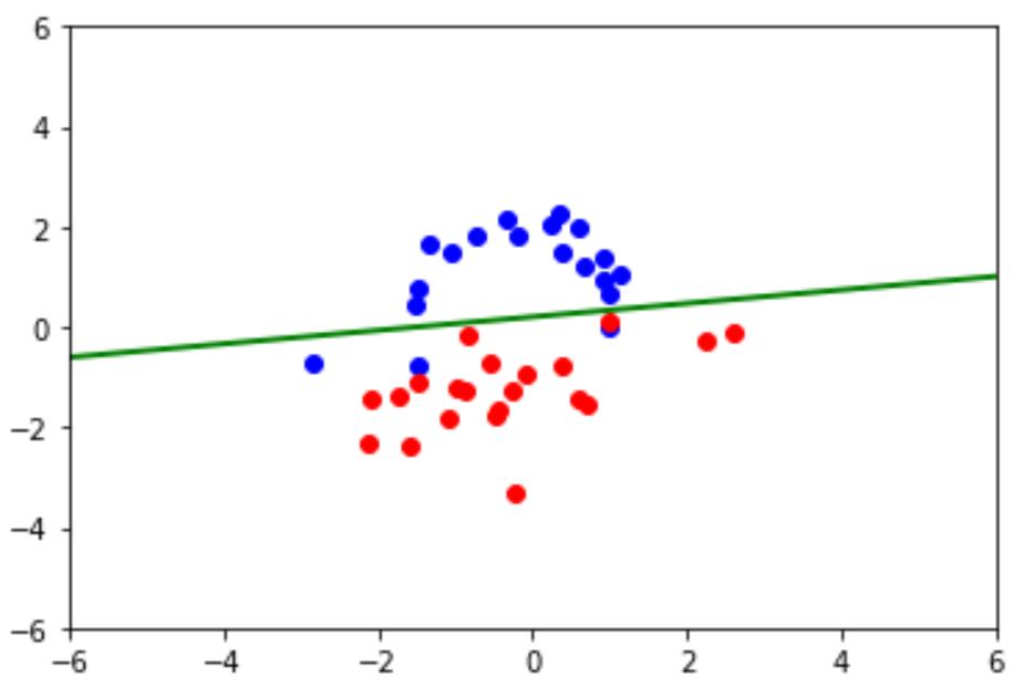
绘图:
def plot_boundary(positive_examples, negative_examples, weights):

   if np.isclose(weights[1], 0):

      if np.isclose(weights[0], 0):

      x = y = np.array([-6, 6], dtype = 'float32')

         else:

            y = np.array([-6, 6], dtype='float32')

            x = -(weights[1] * y + weights[2])/weights[0]

      else:

         x = np.array([-6, 6], dtype='float32')

         y = -(weights[0] * x + weights[2])/weights[1]


   pylab.xlim(-6, 6)

   pylab.ylim(-6, 6)

   pylab.plot(positive_examples[:,0], positive_examples[:,1], 'bo')

   pylab.plot(negative_examples[:,0], negative_examples[:,1], 'ro')

   pylab.plot(x, y, 'g', linewidth=2.0)

   pylab.show()

   plot_boundary(pos_examples,neg_examples,wts)
评估test dataset:
def accuracy(weights, test_x, test_labels):

   res = np.dot(np.c_[test_x,np.ones(len(test_x))],weights)

   return (res.reshape(test_labels.shape)*test_labels>=0).sum()/float(len(test_labels))


   accuracy(wts, test_x, test_labels)
输出:1.0
训练过程:
def train_graph(positive_examples, negative_examples, num_iterations = 100):

   num_dims = positive_examples.shape[1]

   weights = np.zeros((num_dims,1)) # initialize weights

   pos_count = positive_examples.shape[0]

   neg_count = negative_examples.shape[0]

   report_frequency = 15;

   snapshots = []

   for i in range(num_iterations):

      pos = random.choice(positive_examples)

      neg = random.choice(negative_examples)


   z = np.dot(pos, weights)

   if z < 0:

      weights = weights + pos.reshape(weights.shape)


   z = np.dot(neg, weights)

   if z >= 0:

      weights = weights - neg.reshape(weights.shape)

   if i % report_frequency == 0:

      pos_out = np.dot(positive_examples, weights)

      neg_out = np.dot(negative_examples, weights)

      pos_correct = (pos_out >= 0).sum() / float(pos_count)

      neg_correct = (neg_out < 0).sum() / float(neg_count)

      # make correction a list so it is homogeneous to weights list then numpy array accepts

      snapshots.append((np.concatenate(weights),[(pos_correct+neg_correct)/2.0,0,0]))


      return np.array(snapshots)


      snapshots = train_graph(pos_examples,neg_examples)


def plotit(pos_examples,neg_examples,snapshots,step):

   fig = pylab.figure(figsize=(10,4))

   fig.add_subplot(1, 2, 1)

   plot_boundary(pos_examples, neg_examples, snapshots[step][0])

   fig.add_subplot(1, 2, 2)

   pylab.plot(np.arange(len(snapshots[:,1])), snapshots[:,1])

   pylab.ylabel('Accuracy')

   pylab.xlabel('Iteration')

   pylab.plot(step, snapshots[step,1][0], "bo")

   pylab.show()

def pl1(step):
   plotit(pos_examples,neg_examples,snapshots,step)
调用:
interact(pl1, step=widgets.IntSlider(value=0, min=0, max=len(snapshots)-1))
输出:<function __main__.pl1(step)>
感知器的局限性:
感知器是线性分类器,但是不能解决XOR问题
修改:
pos_examples_xor = np.array([[1,0,1],[0,1,1]])

neg_examples_xor = np.array([[1,1,1],[0,0,1]])


snapshots_xor = train_graph(pos_examples_xor,neg_examples_xor,1000)

def pl2(step):
   plotit(pos_examples_xor,neg_examples_xor,snapshots_xor,step)
输入:
interact(pl2, step=widgets.IntSlider(value=0, min=0, max=len(snapshots)-1))
输出:<function __main__.pl2(step)>
精确度75%
其他文章:
-
MNIST实验